Finding flatroofs with QGIS

Emily Selwood is a Software Engineer at the Satellite Applications Catapult, following a Hackathon event in Bristol earlier this year Emily has developed a way of identifying flat roof spaces (that have the potential to be turned into inner-city green spaces) by using programmes that can be downloaded onto your computer. Read, in her own words, how she accomplished this:

A little while ago I attended the Climathon kic event/hackathon in Bristol at my old university. The event was to come up with solutions that could help with pollution in the city. There were not a lot of people who turned up so we formed a single team. The idea we came up with was to create an incentive for people with flat roofs to put plants on them. This meant we needed to be able to find flat roofs in the city. There were suggestions that we could do this with machine learning and looking at satellite images, but I thought we could do this with the Free LIDAR data provided by the environment agency and a few steps of processing.

Assumptions

You have a computer with QGIS installed. You have a few hundred megabytes to a gigabyte of free storage.

Background

There are two sets of data that we are going to need for this. One is the Digital Surface Model (DSM) and the other Digital Terrain Model (DTM). These data sets are generated by an aircraft flying over an area with a laser system on its back. This laser is used to measure the distance from the plane to the surface below. This is then processed to build a height model of the world. The DSM is what is measured by the laser and it includes all the buildings, trees, lamp posts and other things that stick up from the ground. The DTM is further processed to remove these things and leave only the ground.

Downloading the data

The environment agency data website takes a little bit of getting used to but makes sense eventually. You scroll the map and then click on the area you are interested in. This will bring up information at the bottom of the screen about the available data. There are two sets of data: 2 meter and 1 meter. The 1 meter data will give us a better result, though the data will be bigger. The data for each square is split into four parts: North West, North East, South West, South East. If you are interested in a smaller area you can just download the bits you need. For some reason the only way to tell which one you are downloading is the address of the download on the right hand side of the table.

Click the link and download the file. Extract the zip files somewhere. Make sure that each zip file is extracted to its own directory. E.g:

data/
  dsm/
    LIDAR-DSM-1M-ST67nw/
      ...
  dtm/
    LIDAR-DTM-1M-ST67nw/
      ...

Processing

Now to start loading things up in QGIS. The first thing to do is join up the images so they are one image and not lots of small chunks. This will allow us to do less work later. Go to the Raster menu then Miscellaneous and Merge. This will pop up a window that looks like this:

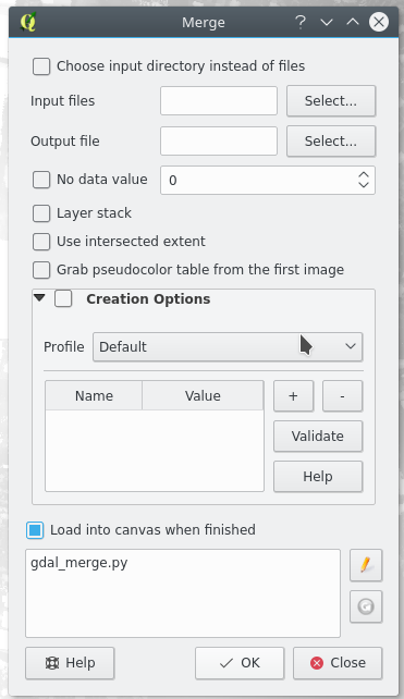
The first thing to do is tick the box for input directories instead of files. This will allow you to select a directory rather than each file individually. Select one of the DSM directories you extracted and set the output file to a tif. I tend to make it the same name as the folder I selected so I know which one is which.

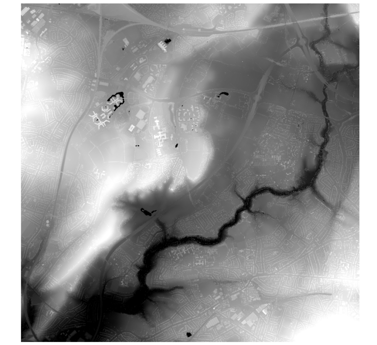
We didn’t need to set anything else, so press the Ok button. When it is done QGIS will open the result in the viewer. You will see a black and white image something like this:

The next step is to re-project this image. The British government uses its own coordinate system. If we want to use this with other things its easier to convert it to a more common projection. Map projections are a very involved topic that is way beyond the scope of this post. If you’re interested there are many good resources out there. To change the coordinate system of the image go to the Raster > Projections > Warp (Reproject) This will bring up a dialog that looks like this:

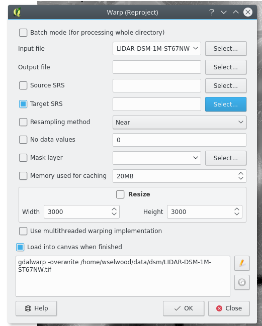
Tick the box next to the Target SRS entry, then press the select button. There should be a long list of possible projections. Find the one labelled WGS 84 or EPSG 4326. On the warp dialog fill in an output name. I usually append _warp or _repo to the name. Press OK and it should load a new image over the top of the old one. This is one of those things that will not appear to be any different, however it will make things easier later.

Next repeat the process for the DTM. Merge the images together and warp them into WGS 84 projection.

Now we have two merged and warped images.

The next step is to subtract the two images. This will leave us with all the things that stick up from the ground. To do this we need to use the Raster Calculator Tool. Select Raster > Raster Calculator from the menu.

This screen is very powerful but it is also intimidating to start with. Upper left are all the images you have loaded up in QGIS so far. On the upper right is the output format options. The important one is the file name, you have to select one or nothing will happen. Also make sure that the output CRS lists WGS 84.

The bottom section is a formula editor. This works a lot like an excel formula but rather than applying to cells it will apply to every pixel in the result image.

What we need to do here is take the DTM away from the DSM. If you double click on a band name in the box on the upper left it will add it to the calculation. Double click on the DSM Image and then click on the minus button in the collection of operators. Finally Double click on the DTM Image.

Hopefully if every thing went well it will say Expression Valid underneath the formula editor. Pick an output file name and press ok.

You should now have an image with a black background and gray and white buildings showing.

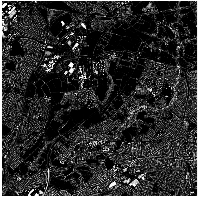
This gives us a pretty good idea of buildings. Some filtering by object size would probably give a good set of building outlines at this point. We, however, want to find flat roofs so we need a couple more steps.

The next thing is to work out how sloped each pixel is. Thankfully QGIS makes this very easy. There is a handy set of tools built in for handling Digital Elevation Model (DEM) data sets, which this is one of. Select Raster > Analysis > DEM (Terrain Models) from the menu.

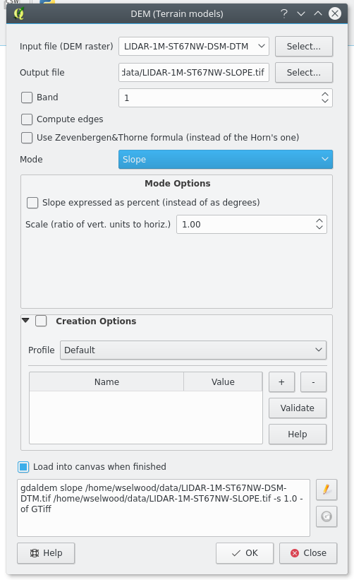
As usual pick an output file name. Make sure you don’t overwrite the source image here, we will need it later. Also make sure the correct Input file is selected if you have more than one open. We need the subtracted image we just generated for the input.

In the mode drop down select Slope then press OK.

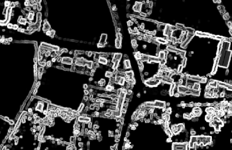
If you zoom in you should find lots of white lines around the walls of buildings (these are vertical slopes) and black between buildings (this is the ground). Some of the buildings will be black in the middle too denoting flat roofs. These are the ones we want to find.

Next we want to find all the places that are off the ground and not sloped. To do this we use the Raster Calculator again. This time we want to create a boolean (zero or one) image where the dsm-dtm image is greater than 3 and the slope image is less than 20 (it’s in degrees).

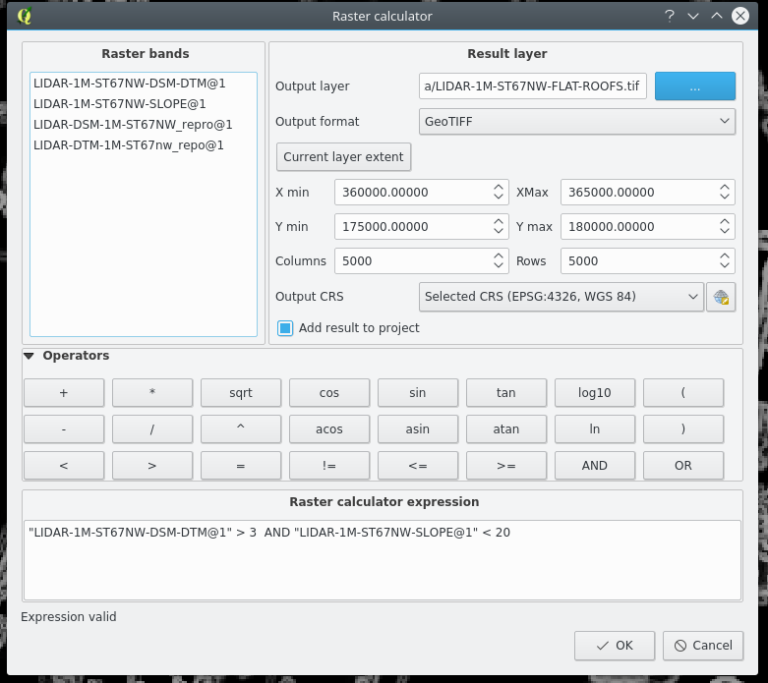
The formula is:

"LIDAR-1M-ST67NW-DSM-DTM@1" > 3 AND "LIDAR-1M-ST67NW-SLOPE@1" < 20

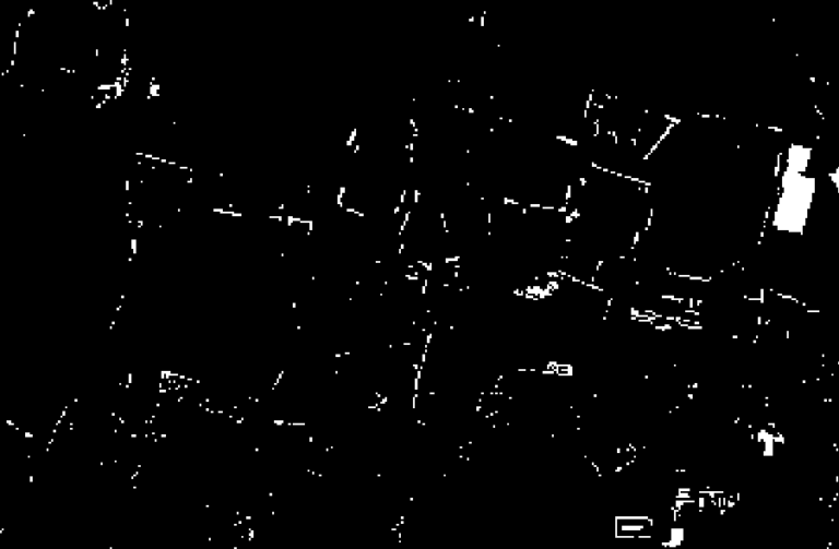
The thresholds for this can be changed if you find they don’t quite work for your area: I was working with Bristol. This will create a purely black and white image. Some bits will be quite speckled with some blobs. If you change the enabled layers in the layers panel you can probably start to work out what something’s are. The thin lines are often the peaks of pitched roofs. Dense Speckles are often trees.

To be able to use this we are going to have to clean up the data. To do that we can use the Sieve tool. Go to Raster > Analysis > Sieve

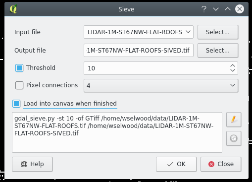
Make sure the right input file is selected then pick an output file. Tick the box next to threshold and enter 25. This is the number of pixels that need to be next to each other to show up in the result. Again this is changeable, but I found this to be a reasonable size that avoided too many long roof peaks showing up in the results. Have a play and see how things come out for your area.

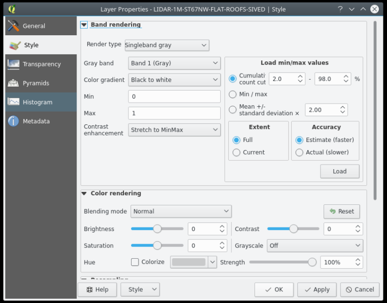
Press ok, you may be lucky here and have a nice image right off the bat. When I did this QGIS picked some very odd values for the colour range so I ended up with an entirely black screen. To fix this double click on the layer in the layer panel and you should get properties appearing. Go to the style section. It should be set to single band gray and there will be min and max boxes. Set the min to 0 and the max to 1.

Now we have a map of all the flat roofs in the area. The last thing that will be useful is to convert this into a vector format that will allow us to do things like overlay on google maps etc. This time we need the polygonize tool. This is under Raster > Conversion > Polygonize (Raster to Vector)

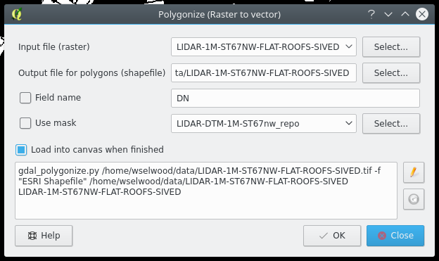
Select the right input file and pick an output file name. This defaults to ESRI shape files (kind of ugly but will do for now) so don’t put an extenson on the output file name. Press OK to start the process. Be aware this can take a while.

When it finishes your map will probably turn a random colour, mine went pink. For some reason a polygon is also drawn around the outside of the image. This is very easy to get rid of however. Right click on the layer and select the Toggle Editing option. Then switch to the Identify Features tool. It should be in the top bar and look like a mouse cursor pointing at an information bubble.

Select somewhere on the map that is background and not another feature. A box should appear on the right. You may need to resize it a bit to be able to see both columns, there should be two. The feature selected should have DN 0 in its labels if it is the border polygon.

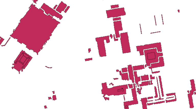
In the tool bars at the top there should be a delete button. It looks like a dustbin. When you click it the background of your area should go white again. Now you just need to save your changes and disable editing. To save the changes to a layer, right click on it and select the Save changes option. Then Toggle Editing again to make sure you don’t do any thing you don’t mean to.

You should end up with something that looks a bit like this:

Conclusion

This turned into a much longer post than I planned however it covers a lot of useful things with the QGIS tools. We learnt to use the Raster Calculator, re-project an image, merge images, sieve an image, and use some of the DEM tools. Finally we also converted an image into polygons.

These are all very useful tools and hopefully you learnt something from this. If you found this interesting or you have any questions please let me know on twitter.